Bob Henson • March 4, 2013 | Snow in February isn’t exactly stop-the-press news. But last month delivered some memorable accumulations and blizzard conditions to several parts of the United States, including New England and the Great Plains. Did these onslaughts catch people off guard?

As a whole, last month’s major snowfalls were amply warned, including the one that walloped New England on February 6–9 and the twin hits to Kansas, Missouri, Oklahoma, and Texas in late February. The National Weather Service (NWS), private firms, and broadcast meteorologists all emphasized that life-threatening conditions could occur and that snow amounts might approach or even top all-time records in some spots. Which, in fact, they did. Some examples:

Heaviest snowfall ever recorded
     •  Portland, Maine (31.9”, February 8–9)

Second heaviest
     •  Concord, New Hampshire (24.0”, February 8–9)
     •  Wichita, Kansas (14.2”, February 20–21)

Third heaviest
     •  Amarillo, Texas (19.0”, February 25)

Fifth heaviest
     •  Boston, Massachusetts (24.9”, February 9)

One reason why these eye-popping snowfall totals didn’t come as a surprise is the growth of ensemble prediction. Little more than a decade ago, U.S. forecasters had access to only a handful of fresh runs of computer models every few hours to guide their snow forecasts. Today, there’s not only a broader range of models, but some of these models are run multiple times, side by side, with small changes in the starting-point conditions that mimic the gaps in our less-than-perfect weather observing network. Such ensembles are helping forecasters deal with such high-impact threats as the “Snowquester” winter storm expected to strike the Washington, D.C., area this week.

Epic snow or epic fail? Let’s check the plumes

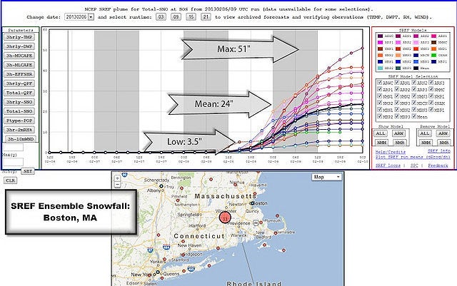
The 23 members of the Short Range Ensemble Forecast system (SREF) predicted a widely varying range of outcomes for Boston three days before the blizzard of February 8–9. The individual model runs produced snowfall amounts that ranged from 3.5 to 51 inches. However, the mean, or average, of an entire ensemble can serve as useful forecast guidance. The observed total in Boston of 24.9 inches ended up very close to the ensemble mean. (Graphic courtesy NOAA.)

When an entire ensemble is plotted on one graph, it’s easy to see the dangers of relying on a single model run. At right is experimental “plume” output from the Short Range Ensemble Forecast system, operated by NOAA’s Storm Prediction Center.

SREF carries out 22 model runs every six hours. All are based on variations of the Weather Research and Forecasting model (WRF), a multiagency effort in which NCAR has played a major role. Click on “SREF Info” on the plumes page for more about the plumes.

Several days before Boston’s big snow, SREF showed the potential for massive accumulations—as well as for a bust. As shown in the graphic above, the predictions varied from a modest 3.5 inches to a snow lover’s dream of 51 inches.

What’s a forecaster to do? Sometimes—though not always—the average of a large ensemble is the best route. The assumption here is that errors would tend to be equally distributed on either side of the eventual outcome. In the case of Boston, the ensemble mean, or average, shown in the graphic (24 inches) came less than an inch short of the final total, an impressive forecast indeed. It’s also clear that relying on a handful of individual model runs, which was par for the course until recent years, can produce a forecast destined to be spectacularly wrong.

Ensembles aren’t magic, though. Sometimes a subtle twist in unfolding weather whose importance will grow over time goes unseen by all ensemble members. As a result, most or all of the members may err in the same direction. Or a weather situation may play into the known biases of the particular models that make up a given ensemble.

A savvy forecaster will keep such circumstances in mind while watching to see how the spread of ensemble solutions behaves over successive model runs as a weather event gets closer in time. If the spread stays wide, there may be more inherent uncertainty in the atmosphere’s behavior for this storm. If the spread begins to shift toward the high or low end, then the current ensemble mean might not be the best forecast. 

Getting edgy about snow totals

One complication in snow forecasting is that accumulations depend critically on the snow-to-liquid ratio, or the amount of snowfall per unit of moisture. This value is shaped by the temperature and moisture amounts at the heights and locations where the snow is being made. A commonly cited average for lower elevations in the United States is 12-to-1 (1 inch of water yielding 12 inches of snow). But the ratios vary strongly by region, and even from storm to storm in a given place. Fluffy dendrites—what we picture as classically shaped snowflakes—may have ratios of 20-to-1 or higher.

Moreover, the edges of a big snowstorm are still notoriously difficult areas to forecast. Sometimes only a few miles can separate heavy rain from heavy snow, with a highly dynamic transition zone in between. This is a familiar phemonenon near the New England coast, but it can also occur well inland.

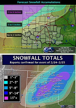
Five days in advance of the February 25 blizzard, forecasters at the Oklahoma City NWS office provided a heads-up that major snow could be expected across the northwest half of the state (top graphic). The forecasted amounts rose as the storm took shape, with final accumulations (bottom graphic) topping 18 inches in parts of far northwest Oklahoma and the Texas Panhandle. (Top graphic courtesy NWS/Norman; bottom graphic courtesy NWS/Amarillo.)

Oklahoma City found itself on the wet side of such a transition zone last week. Forecasters correctly pegged a dramatic transition from extremely heavy snow and gale-force winds in far northwest Oklahoma to lighter but still hazardous amounts toward the center of the state (see top graphic at left), with rain predominating farther to the southeast. The night before the storm, the SREF plume (not shown) called for 1 to 10 inches in Oklahoma City, with an ensemble mean of about 4 inches.

But the rain/snow line stayed a few tens of miles further west than expected during the height of the storm (see bottom graphic at left), which left Oklahoma City with less than an inch of snowfall, outside the range of all SREF ensemble members from the night before. Even though the regional forecast was excellent, weathercasters who’d emphasized the local risks (more or less in line with NWS forecasts and warnings) found themselves subjected to biting critiques.

Similar issues may occur in this week’s Snowquester event, with the rain/snow transition line expected to set up near or just east of Washington, D.C. That could give the city’s western suburbs 6 inches or more of snow while the eastern suburbs get little or nothing. Not surprisingly, the most recent SREF plume at this writing (produced late Monday morning, March 4) show predicted amounts at Washington’s Reagan National Airport ranging wildly—from around 5 to 23 inches.

In fairness, predicting snowfall amounts has never been for the faint of heart. If a forecast calls for 3 to 6 inches of snow, and people wake up to find a foot on the ground, the mistake is painfully obvious. With rainfall, the forecast isn’t so easy for a layperson to verify. If a deluge of 5 inches follows a prediction of 2 to 3 inches of rain, it takes more than a glance out the window to confirm that the rainfall was heavier than expected.

It's also worth noting that measuring snow accurately is a challenge of its own, as discussed in this AtmosNews post on March 18.

More resolution, more often

Higher-resolution, high-frequency models may soon provide more help to pin down features like the ones that robbed Oklahoma City of its expected snowfall.

In 2011 the NWS introduced the Rapid Refresh model (NOAA/NCEP RAP). Based on the research-oriented WRF model, it’s run every hour and extends out to 18 hours. (See graphics produced by NCAR’s Real-time Weather Data service.) The High-Resolution Rapid Refresh (HRRR) brings the RAP's 13-kilometer resolution down to 3 km, which is sharp enough to depict and track individual thunderstorms and other similarly sized features. Though still classified as experimental until its scheduled 2015 adoption by NWS, the HRRR is available to forecasters and run hourly by NOAA’s Earth System Research Laboratory.

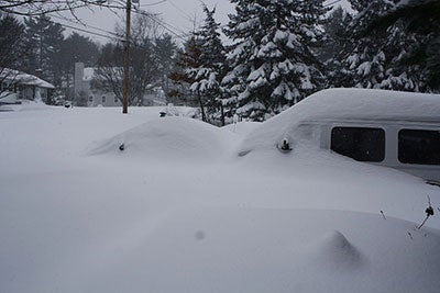
Northwest of Boston, the town of Billerica, Massachusetts, was hammered by more than two feet of snow on February 8–9, 2013. (Wikimedia Commons photo by Game Freak2600.)

All of the big winter events noted above were captured several days in advance by longer-range forecast models. However, there was some noteworthy international disagreement beyond three or so days. The flagship model of the European Centre for Medium-Range Weather Forecasts (ECMWF) was the first to consistently project that the February 8–9 storm would be close enough to the Northeast coast to cause major problems. The ECMWF called for a major New England storm as much as a week in advance, while the NWS’s Global Forecast System model (GFS) took several more days to lock into a big-snow forecast.

This hits the same bell rung by Hurricane Sandy, when the ECMWF landed on a consistent forecast for major Northeast impacts several days ahead of the GFS. Interestingly, both the Sandy superstorm and the blizzard involved a moisture-laden system from low latitudes getting swept up by an upper-level storm diving into the eastern U.S.

“Seperately, the two waves that preceded the blizzard were not that impressive,” says Ed Szoke (Cooperative Institute for Research in the Atmosphere). "But the southern wave carried a lot of subtropical moisture. It’s possible that latent heat released from that moisture was an important factor in how the blizzard developed.”

Cliff Mass (University of Washington) recently took a closer look at ECMWF-versus-GFS performance during the February 8–9 blizzard, as well as the broader implications of the two models’ contrasting behavior.

The European model also sounded the earliest alarm for the impending Snowquester, according to Szoke. “The ECMWF was all over this as a big storm for the mid-Atlantic, focused in the North Carolina/Virginia area, while the GFS and other models tended to take the storm out to sea before deepening it. Eventually the GFS came on board, but all of the models have shifted north a bit toward the D.C. area.”

See all News